
Communication System Engineering (MIE 113)
Welcome to this comprehensive study material and blog post on the foundational theoretical concepts in communications systems engineering. This unit is designed for 20 hours of learning, breaking down complex topics into digestible explanations, examples, and visuals. Whether you're a student or enthusiast, use this as a guide for self-paced learning. We've included animations, diagrams, and recommended videos for better understanding.
Topic 1: Elements of a Generic Communications System/Digital Communication System and Various Issues Associated with Each Element
First, let's look at the elements of a generic communication system. This is like the blueprint for how information travels from sender to receiver. The key components are: the information source (e.g., voice or data), transmitter (encodes and modulates the signal), channel (medium like air or cable, prone to noise), receiver (demodulates and decodes), and destination (user or device).
In a digital system, we add analog-to-digital conversion at the start and digital-to-analog at the end. Issues include: noise in the channel degrading signals, bandwidth limitations restricting data rate, and power constraints in transmitters.
Example: In a phone call, your voice (source) is digitized, transmitted over wires (channel), and reconstructed at the receiver. If noise interferes, you hear static—that's a channel issue.
Visual: Block Diagram

Basic Communication System Explained | Block Diagram, Elements & Classification
Recommended Animation/Video:
Further Reading: rfwireless-world.com, boardmix.com
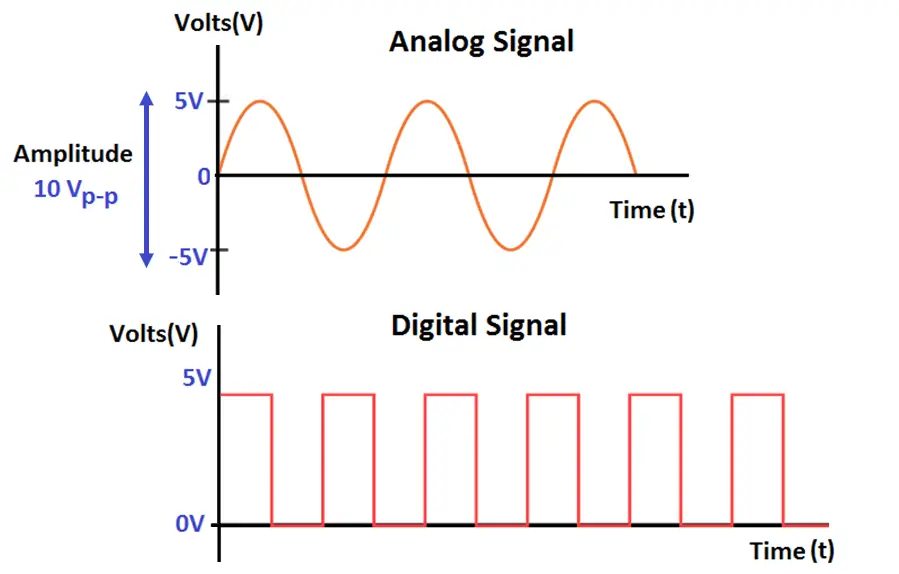
Topic 2: Comparison Between Analog and Digital Communications Systems
Now, comparing analog and digital systems. Analog transmits continuous signals (like radio waves varying smoothly), while digital uses discrete bits (0s and 1s). Analog is simpler and cheaper but susceptible to noise—distortions accumulate. Digital is more robust with error correction, easier to encrypt, and integrates with computers, but requires more bandwidth initially.
Advantages of digital: Better noise immunity, multiplexing ease, and data compression. Drawbacks: Higher complexity in conversion. Example: FM radio (analog) vs. streaming music (digital)—digital sounds clearer over long distances.
Visual: Side-by-Side Comparison Diagram
How does an analog signal differ from a continuous signal and a ...
Recommended Animation/Video:
Further Reading: geeksforgeeks.org, youtube.com
Topic 3: Nyquist Sampling Theorem for Analog to Digital Conversion
The Nyquist sampling theorem is crucial for digitizing analog signals without loss. It states: To accurately reconstruct a signal, sample it at least twice the highest frequency component ($f_s \geq 2f_{max}$). If undersampled, aliasing occurs—high frequencies masquerade as low ones.
Example: Audio CDs sample at 44.1 kHz for human hearing up to 20 kHz (2*20k=40k, with margin). Violate it, and music sounds distorted.
Visual: Illustration with Waveform

Nyquist Sampling Theorem - GeeksforGeeks
Recommended Animation/Video:
Further Reading: geeksforgeeks.org, sciencedirect.com
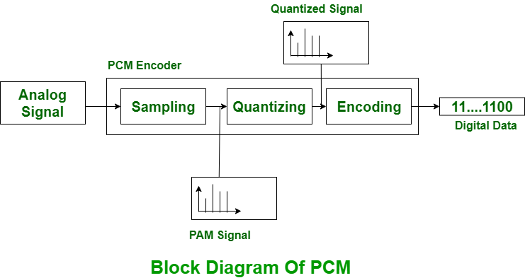
Topic 4: Waveform Coding Techniques: PCM, DPCM, ADPCM, DM, ADM
Waveform coding digitizes analog signals. PCM (Pulse Code Modulation) samples, quantizes, and encodes—basic but bandwidth-heavy. DPCM (Differential PCM) encodes differences, reducing bits. ADPCM adapts quantization for efficiency. DM (Delta Modulation) uses 1-bit for changes—simple but slope overload prone. ADM adapts step size to avoid that.
Example: PCM in telephony (8-bit, 8kHz); DM in low-bitrate voice.
Visual: Waveforms Comparison
(No suitable image found; refer to recommended video for visualization.)
Recommended Animation/Video:
Further Reading: totalecer.blogspot.com, codes.pratikkataria.com
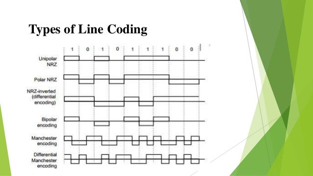
Topic 5: Baseband Shaping for Data Transmission: Unipolar, Polar, Bipolar Signals - NRZ, RZ, Manchester, AMI Format
Baseband shaping formats digital data for transmission. Unipolar: 0/low voltage. Polar: Positive/negative. Bipolar: Alternating polarities.
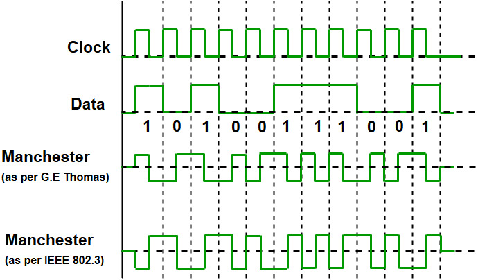
Formats: NRZ (Non-Return-to-Zero)—level constant; RZ (Return-to-Zero)—pulses return to zero; Manchester—self-clocking with mid-bit transition; AMI (Alternate Mark Inversion)—alternates polarity for balance.
Example: Ethernet uses Manchester for clock recovery.
Visual: Signal Waveforms

Recommended Animation/Video:
Further Reading: technologyuk.net, vedveethi.co.in
Topic 6: Analog Modulation Techniques - Time Domain and Frequency Domain Analysis
Analog modulation varies carrier with message. AM (Amplitude): Varies amplitude—simple but noise-prone. FM (Frequency): Varies frequency—better noise resistance.
Time domain: Waveform views. Frequency domain: Spectra showing sidebands.
Example: AM radio vs. FM radio.
Visual: Graphs
(No suitable image found; refer to recommended video for visualization.)
Recommended Animation/Video:
Further Reading: geeksforgeeks.org, tutorialspoint.com
Topic 7: Digital Modulation Techniques
Digital modulation: ASK (Amplitude Shift Keying)—on/off amplitude; FSK (Frequency Shift)—freq switches; PSK (Phase Shift)—phase changes; QAM (Quadrature Amplitude)—combines amplitude/phase.
Evaluated by bandwidth efficiency, power, BER.
Visual: Constellations/Diagrams
.png)
Recommended Animation/Video:
Further Reading: salimwireless.com, eecs.yorku.ca
Topic 8: Evaluation of System Performance: SNR and BER
SNR (Signal-to-Noise Ratio): Power ratio, higher better. BER (Bit Error Rate): Error fraction, lower better. SNR affects BER—higher SNR, lower BER.
Visual: Graph
Comparison of the BER vs SNR performance graph for | Download ...
Recommended Animation/Video:
Further Reading: researchgate.net, researchgate.net
Topic 9: Information and Entropy, Source Coding Theorem, Huffman Coding
Information: Uncertainty measure. Entropy: Average info per symbol. Source Coding Theorem: Minimum bits needed = entropy.
Huffman: Variable-length codes, frequent symbols short codes.
Visual: Tree

Recommended Animation/Video:
Further Reading: en.wikipedia.org, geeksforgeeks.org
Topic 10: Shannon’s Channel Capacity Theorem
$C = B \log_2(1 + \text{SNR})$—This formula gives the maximum theoretical error-free data rate (C) given bandwidth (B) and Signal-to-Noise Ratio (SNR). It defines the fundamental limits of communication due to noise and bandwidth.
Visual: Formula/Graph
experimental physics - Negative SNR and Shannon–Hartley theorem ...
Recommended Animation/Video:
Further Reading: ingenu.com, sciencedirect.com
Topic 11: Error-Control Coding: Rationale for Coding and Types of Codes, Linear Block Codes, Error Detection and Correction, Convolutional Codes
Coding adds redundancy (extra bits) to the data stream to allow the receiver to detect and/or correct errors caused by channel noise. Block codes (e.g., Hamming) group bits into blocks for coding; convolutional codes use shift registers for streaming data.
Rationale: Combat noise. Linear block: Uses parity checks for easy encoding/decoding. Convolutional: Typically decoded using the Viterbi algorithm (Trellis decoding).
Visual: Diagrams
Structural representation of linear block code. Linear Block Codes ...
Recommended Animation/Video:
Further Reading: engineerstutor.com, wikiwand.com
Topic 12: Multiplexing, Emerging Trends in Modulation, Error Control Coding, and Multiplexing
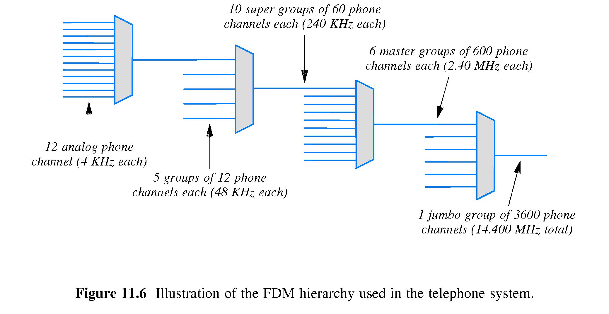
Multiplexing shares a single communication channel among multiple users: TDM (Time Division Multiplexing—time slots), FDM (Frequency Division Multiplexing—frequency bands), CDM (Code Division Multiplexing—unique codes).
Emerging Trends: OFDM (Orthogonal Frequency-Division Multiplexing—multi-carrier system used in 4G/5G), advanced FEC like LDPC (Low-Density Parity-Check), and NOMA (Non-Orthogonal Multiple Access) multiplexing.
Visual: Diagrams

14. Understanding Multiplexing: FDM, TDM, CDM, and WDM Explained!
Exam Questions & Answers (Collapsible Practice Section)
Use the collapsible sections below to test your knowledge on the topics covered above. Click to reveal the answer.
Communication Systems Study Material
1(a) Earlier communication systems were largely analog. Some of the systems are still analog. But the majority of the communication systems have been digitized and the remaining are in the process of digitization. Give examples to substantiate these statements. Why do you think this analog to digital change happened and is still happening?
Analog vs Digital Communication
Early systems were analog (continuous signals), but most have transitioned to digital (discrete binary) for better quality and efficiency. Some legacy systems remain analog, while others are being upgraded.
Examples
- Telephone: From analog PSTN to digital VoIP (e.g., Skype, Zoom).
- Television: Analog (NTSC/PAL) to Digital TV (HD, 4K).
- Radio: AM/FM analog to Digital (DAB, HD Radio, streaming).

Reasons for Transition
- Better noise immunity and signal regeneration.
- Higher efficiency (compression, more channels).
- Integration with digital devices, encryption, error correction.
- Support for modern services (internet, 5G, IoT).
1B: Analog to digital change over requires A/D conversion of analog baseband signal. Explain one of the widely used such techniques and derive the formula for the data rate of the digital output.
Pulse Code Modulation (PCM)
PCM is a widely used A/D technique: Sampling → Quantization → Encoding.
- Sampling at fs ≥ 2 × f_max (Nyquist).
- Quantization to 2^n levels.
- Encoding each sample to n bits.
Data Rate Derivation
Data rate R = f_s × n bps
(samples/second × bits/sample)
Example: Voice (4 kHz max) → fs = 8 kHz, n=8 → R=64 kbps.
2.a: What do you mean by a line code? Where is a line code used? List all the desirable characteristics of a line code. For a data sequence 110110, draw the waveform for NRZ, RZ, Manchester, AMI.
Line Code
A line code encodes binary data into waveforms for baseband transmission.
Uses
- Ethernet, USB, digital telephony, storage.
Desirable Characteristics
- No DC component
- Self-synchronization
- Error detection
- Bandwidth efficiency
- Power efficiency
- Noise immunity
- Transparency
- Low complexity
Waveforms for 110110
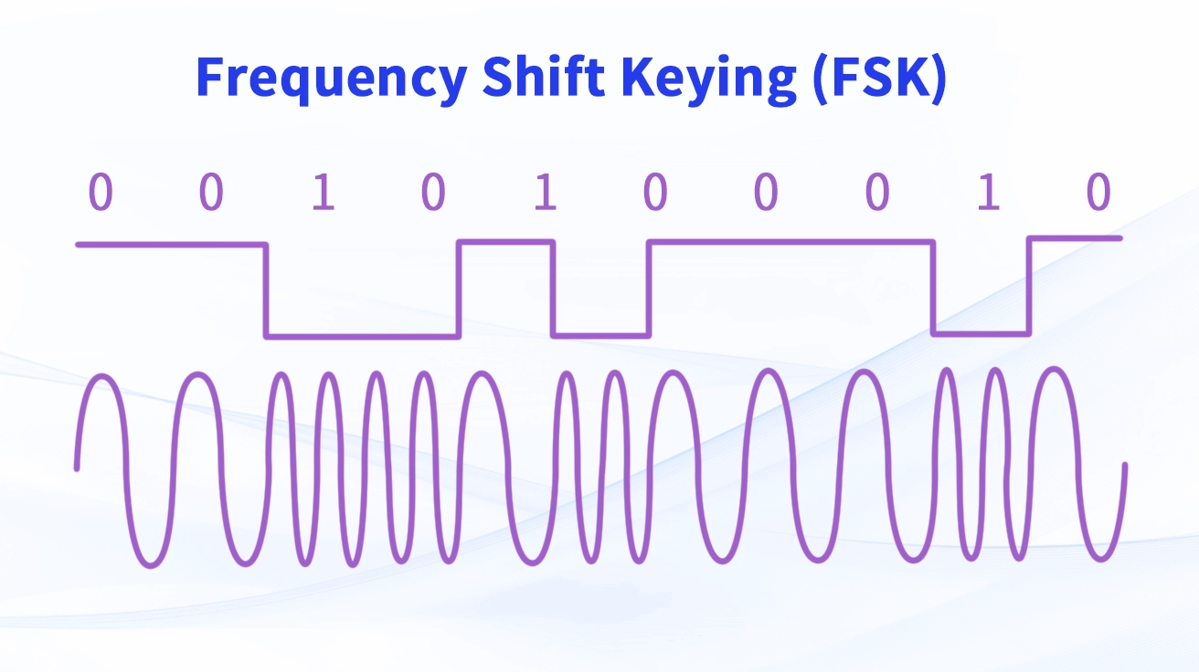
2B: Draw waveform for the data sequence 10101 using ASK, FSK and PSK.
Digital Modulation Waveforms for 10101
ASK: Amplitude changes (high for 1, low/none for 0).
FSK: Frequency changes (two frequencies).
PSK: Phase shifts (e.g., 0° for 0, 180° for 1).

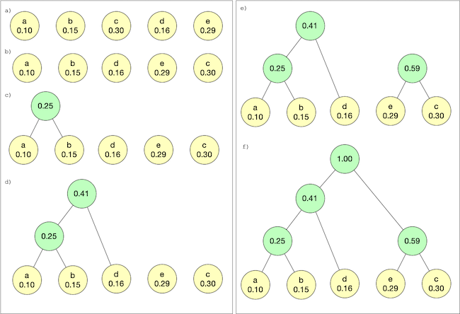
3a: Consider a discrete source generating five alphabets with probabilities (0.35, 0.25, 0.20, 0.10, 0.10). Find the Huffman code, entropy and coding efficiency for this source.
Huffman Coding
Symbols: A(0.35), B(0.25), C(0.20), D(0.10), E(0.10)
Step-by-step tree: Combine lowest probabilities repeatedly.
Possible Huffman Codes (one variant):
- A: 0 (length 1)
- B: 10 (2)
- C: 110 (3)
- D: 1110 (4)
- E: 1111 (4)
Average length ≈ 2.05 bits/symbol
Entropy H = -∑ p log₂p ≈ 2.13 bits/symbol
Efficiency = H / average length ≈ 96-98% (very high)
Video: Huffman Coding Greedy Method
3B: Define modulation, compare AM, PM and FM.
Modulation: Process of varying a carrier signal's parameter (amplitude, frequency, phase) with the message signal for efficient transmission.
| Parameter | AM | FM | PM |
|---|---|---|---|
| Varied | Amplitude | Frequency | Phase |
| Noise Immunity | Poor | Good | Best |
| Bandwidth | 2×message BW | Large (Carson's rule) | Similar to FM |
| Complexity | Simple | Moderate | Complex |
| Applications | Radio broadcasting | FM radio, TV sound | Indirect FM, digital |

Video: Comparison of AM, FM and PM
3C: Write short note on ADPCM.
ADPCM (Adaptive Differential PCM): Variant of DPCM where quantization step size adapts to signal variations, reducing bit rate while maintaining quality.
Encodes difference from predicted value; step size adjusts dynamically.
Used in speech coding (e.g., G.726 at 16-40 kbps), VoIP.
Advantages: Lower bitrate than PCM, better than fixed DPCM.
Video: ADPCM Explanation
4a: Carry out a power budget analysis for the given long haul optical fiber link and state whether this system is good.
Link length=185 km, Tx Power=1 mW (0 dBm), α=0.25 dB/km, Splices=46 (0.1 dB each), Connectors=2 (0.2 dB each), Rx Sensitivity=-28 dBm, Margin=6 dB, D=18 ps/nm-km.
Power Budget Calculation
Fiber loss = α × L = 0.25 × 185 = 46.25 dB
Splice loss = 46 × 0.1 = 4.6 dB
Connector loss = 2 × 0.2 = 0.4 dB
Total loss = 46.25 + 4.6 + 0.4 = 51.05 dB
Received power = Tx power - Total loss = 0 - 51.05 = -51.05 dBm
Available margin = Rx sensitivity - Received power = -28 - (-51.05) = 23.05 dB
Required margin = 6 dB → Actual margin 23.05 dB > 6 dB → System is good (plenty of margin).
Dispersion not critical for power budget (affects signal quality, not power).
4b: Draw the generalized architecture of a GSM cellular system and explain the functions and features of various components.
GSM components: MS (Mobile Station), BSS (BTS + BSC), NSS (MSC, HLR, VLR, AuC, EIR), OSS.

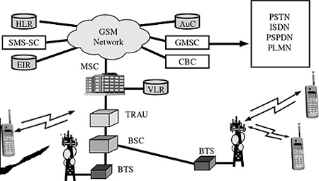
Key functions: BTS (radio transmission), BSC (handover/control), MSC (switching), HLR/VLR (subscriber data).
Video: GSM Architecture Explained
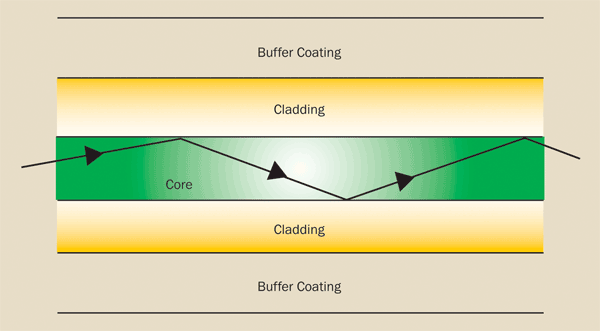
5a: What are the advantages of optical fiber with respect to its construction, theory of light propagation, types, and transmission characteristics.
Advantages
- High bandwidth & speed
- Low attenuation (long distances)
- Immune to EMI
- Lightweight, small size
- Secure (hard to tap)
- Types: Single-mode (long haul), Multi-mode (short)
- Propagation: Total Internal Reflection
Video: Optical Fiber Advantages
5b: What do you mean by multiplexing? Compare TDM and FDM systems. How do you calculate the channel capacity of a transmission medium?
Multiplexing: Combining multiple signals over one channel.
| TDM | FDM | |
|---|---|---|
| Signal Type | Digital/Analog | Analog |
| Division | Time slots | Frequency bands |
| Synchronization | Required | Not needed |
| Crosstalk | Low | Possible (guard bands) |
| Applications | PCM telephony | Radio, TV |
Channel Capacity (Shannon)
C = B log₂(1 + SNR) bps
(B = bandwidth, SNR = signal-to-noise ratio)
Video: TDM vs FDM